Building Regression Model using Keras: Part 1

In part 1 of this notebook, a regression model will be built using Keras deep learning framework to predict the compressive strength of concrete, based on its ingredients. The model will be trained several times with different network properties such as the number of epochs and hidden layers, to increase the model accuracy.

Credit: IBM Cognitive Class

Building a Concrete Compressive Strength Model using Keras Framework

Concrete Ingredients:

1. Cement
2. Blast Furnace Slag
3. Fly Ash
4. Water
5. Superplasticizer
6. Coarse Aggregate
7. Fine Aggregate
8. Age

1. OBTAIN - Obtain Data from its Source.

First lets download the data and stored in pandas dataframe.

import pandas as pd
import numpy as np

import matplotlib.pyplot as plt
import seaborn as sns

url = 'https://s3-api.us-geo.objectstorage.softlayer.net/cf-courses-data/CognitiveClass/DL0101EN/labs/data/concrete_data.csv'

df = pd.read_csv(url)

df.head()

	Cement	Blast Furnace Slag	Fly Ash	Water	Superplasticizer	Coarse Aggregate	Fine Aggregate	Age	Strength
0	540.0	0.0	0.0	162.0	2.5	1040.0	676.0	28	79.99
1	540.0	0.0	0.0	162.0	2.5	1055.0	676.0	28	61.89
2	332.5	142.5	0.0	228.0	0.0	932.0	594.0	270	40.27
3	332.5	142.5	0.0	228.0	0.0	932.0	594.0	365	41.05
4	198.6	132.4	0.0	192.0	0.0	978.4	825.5	360	44.30

Let’s check the shape of the dataframe:

df.shape

(1030, 9)

It has 1030 rows and 9 columns.

2. SCRUB - Clean / Preprocess Data to Format that Machine Understand.

df.isnull().sum()

Cement                0
Blast Furnace Slag    0
Fly Ash               0
Water                 0
Superplasticizer      0
Coarse Aggregate      0
Fine Aggregate        0
Age                   0
Strength              0
dtype: int64

df.dtypes

Cement                float64
Blast Furnace Slag    float64
Fly Ash               float64
Water                 float64
Superplasticizer      float64
Coarse Aggregate      float64
Fine Aggregate        float64
Age                     int64
Strength              float64
dtype: object

The data looks very clean; no missing data and all data is in numerical form.

Nothing much here, lets move to our next step!

3. EXPLORE - Find Significant Patterns and Trends using Statistical Method.

df.describe()

	Cement	Blast Furnace Slag	Fly Ash	Water	Superplasticizer	Coarse Aggregate	Fine Aggregate	Age	Strength
count	1030.000000	1030.000000	1030.000000	1030.000000	1030.000000	1030.000000	1030.000000	1030.000000	1030.000000
mean	281.167864	73.895825	54.188350	181.567282	6.204660	972.918932	773.580485	45.662136	35.817961
std	104.506364	86.279342	63.997004	21.354219	5.973841	77.753954	80.175980	63.169912	16.705742
min	102.000000	0.000000	0.000000	121.800000	0.000000	801.000000	594.000000	1.000000	2.330000
25%	192.375000	0.000000	0.000000	164.900000	0.000000	932.000000	730.950000	7.000000	23.710000
50%	272.900000	22.000000	0.000000	185.000000	6.400000	968.000000	779.500000	28.000000	34.445000
75%	350.000000	142.950000	118.300000	192.000000	10.200000	1029.400000	824.000000	56.000000	46.135000
max	540.000000	359.400000	200.100000	247.000000	32.200000	1145.000000	992.600000	365.000000	82.600000

plt.figure(figsize=(12, 5))
correlation_matrix = df.corr()
sns.heatmap(correlation_matrix, annot=True)
plt.show()

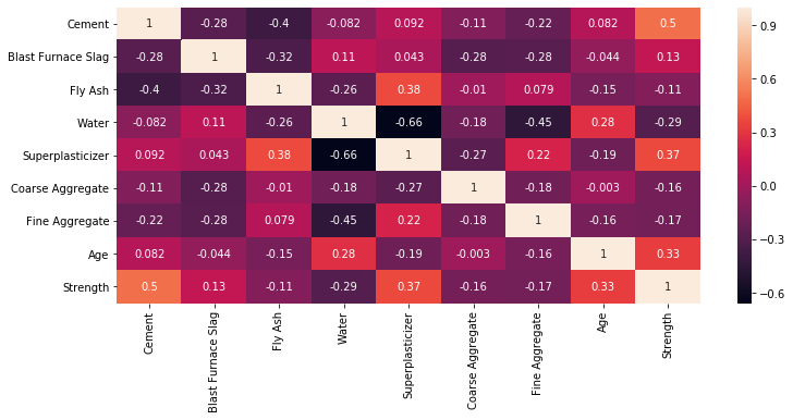
As our objective is mainly to build the model, we will just touch a few in this EDA (exploratory data analysis) section.

4. MODEL - Construct Model to Predict and Forecast.

The part where the magic happens.

Split Data to Predictors and Target

X = df.iloc[:,:-1]
X.head()

	Cement	Blast Furnace Slag	Fly Ash	Water	Superplasticizer	Coarse Aggregate	Fine Aggregate	Age
0	540.0	0.0	0.0	162.0	2.5	1040.0	676.0	28
1	540.0	0.0	0.0	162.0	2.5	1055.0	676.0	28
2	332.5	142.5	0.0	228.0	0.0	932.0	594.0	270
3	332.5	142.5	0.0	228.0	0.0	932.0	594.0	365
4	198.6	132.4	0.0	192.0	0.0	978.4	825.5	360

y = df.iloc[:,-1]
y.head()

0    79.99
1    61.89
2    40.27
3    41.05
4    44.30
Name: Strength, dtype: float64

Save number of feature columns, n_cols to use later in model development.

n_cols = X.shape[1]
n_cols

8

Importing SKLEARN and KERAS Libraries

from sklearn.model_selection import train_test_split
from sklearn.metrics import mean_squared_error
from sklearn.metrics import r2_score

import keras

from keras.models import Sequential
from keras.layers import Dense

Using TensorFlow backend.

Building the Model

A. BASELINE MODEL

Network Properties:

• Hidden Layer: 1
• Nodes: 10
• Activation Function: ReLU
• Optimizer: Adam
• Loss Function: Mean Squared Error
• Epochs: 50

mse_A = []
r2_A = []

for i in range(50):
    
    #Split Data to Train and Test Set
    X_train, X_test, y_train, y_test = train_test_split(X, y, test_size = 0.3)

    #Create model
    model = Sequential()
    model.add(Dense(10, activation='relu', input_shape=(n_cols,)))
    model.add(Dense(1))

    #Compile model
    model.compile(optimizer='adam', loss='mean_squared_error')

    #fit the model
    model.fit(X_train, y_train, epochs=50, verbose=0)

    #predict output on test set
    y_pred = model.predict(X_test)
    
    mse_A.append(mean_squared_error(y_test, y_pred))
    r2_A.append(r2_score(y_test, y_pred))

print('mse_Mean: {:.2f}'.format(np.mean(mse_A)))
print('mse_StdDev: {:.2f}'.format(np.std(mse_A)))

mse_Mean: 421.94
mse_StdDev: 595.59

print('R^2_Mean: {:.2f}'.format(np.mean(r2_A)))
print('R^2_StdDev: {:.2f}'.format(np.std(r2_A)))

R^2_Mean: -0.54
R^2_StdDev: 2.20

B. MODEL WITH NORMALIZED DATA

Network Properties:

• Hidden Layer: 1
• Nodes: 10
• Activation Function: ReLU
• Optimizer: Adam
• Loss Function: Mean Squared Error
• Epochs: 50

Model is retrain with normalized data.

X_norm = (X - X.mean()) / X.std()
X_norm.head()

	Cement	Blast Furnace Slag	Fly Ash	Water	Superplasticizer	Coarse Aggregate	Fine Aggregate	Age
0	2.476712	-0.856472	-0.846733	-0.916319	-0.620147	0.862735	-1.217079	-0.279597
1	2.476712	-0.856472	-0.846733	-0.916319	-0.620147	1.055651	-1.217079	-0.279597
2	0.491187	0.795140	-0.846733	2.174405	-1.038638	-0.526262	-2.239829	3.551340
3	0.491187	0.795140	-0.846733	2.174405	-1.038638	-0.526262	-2.239829	5.055221
4	-0.790075	0.678079	-0.846733	0.488555	-1.038638	0.070492	0.647569	4.976069

mse_B = []
r2_B = []

for i in range(50):
    
    #Split Data to Train and Test Set
    X_train, X_test, y_train, y_test = train_test_split(X_norm, y, test_size = 0.3)

    #Create model
    model = Sequential()
    model.add(Dense(10, activation='relu', input_shape=(n_cols,)))
    model.add(Dense(1))

    #Compile model
    model.compile(optimizer='adam', loss='mean_squared_error')

    #fit the model
    model.fit(X_train, y_train, epochs=50, verbose=0)

    #predict output on test set
    y_pred = model.predict(X_test)
    
    mse_B.append(mean_squared_error(y_test, y_pred))
    r2_B.append(r2_score(y_test, y_pred))

print('mse_Mean: {:.2f}'.format(np.mean(mse_B)))
print('mse_StdDev: {:.2f}'.format(np.std(mse_B)))

mse_Mean: 372.05
mse_StdDev: 104.26

print('R^2_Mean: {:.2f}'.format(np.mean(r2_B)))
print('R^2_StdDev: {:.2f}'.format(np.std(r2_B)))

R^2_Mean: -0.32
R^2_StdDev: 0.37

C. MODEL WITH 100 EPOCHS

Network Properties:

• Hidden Layer: 1
• Nodes: 10
• Activation Function: ReLU
• Optimizer: Adam
• Loss Function: Mean Squared Error
• Epochs: 100

Model is retrained with 100 epochs.

mse_C = []
r2_C = []

for i in range(50):
    
    #Split Data to Train and Test Set
    X_train, X_test, y_train, y_test = train_test_split(X_norm, y, test_size = 0.3)

    #Create model
    model = Sequential()
    model.add(Dense(10, activation='relu', input_shape=(n_cols,)))
    model.add(Dense(1))

    #Compile model
    model.compile(optimizer='adam', loss='mean_squared_error')

    #fit the model
    model.fit(X_train, y_train, epochs=100, verbose=0)

    #predict output on test set
    y_pred = model.predict(X_test)
    
    mse_C.append(mean_squared_error(y_test, y_pred))
    r2_C.append(r2_score(y_test, y_pred))

print('mse_Mean: {:.2f}'.format(np.mean(mse_C)))
print('mse_StdDev: {:.2f}'.format(np.std(mse_C)))

mse_Mean: 162.55
mse_StdDev: 16.92

print('R^2_Mean: {:.2f}'.format(np.mean(r2_C)))
print('R^2_StdDev: {:.2f}'.format(np.std(r2_C)))

R^2_Mean: 0.41
R^2_StdDev: 0.05

D. MODEL WITH 3 HIDDEN LAYERS

Network Properties:

• Hidden Layers: 3
• Nodes: 10
• Activation Function: ReLU
• Optimizer: Adam
• Loss Function: Mean Squared Error
• Epochs: 100

Model is retrained with 3 hidden layers.

mse_D = []
r2_D = []

for i in range(50):
    
    #Split Data to Train and Test Set
    X_train, X_test, y_train, y_test = train_test_split(X_norm, y, test_size = 0.3)

    #Create model
    model = Sequential()
    model.add(Dense(10, activation='relu', input_shape=(n_cols,)))
    model.add(Dense(10, activation='relu'))
    model.add(Dense(10, activation='relu'))
    model.add(Dense(1))

    #Compile model
    model.compile(optimizer='adam', loss='mean_squared_error')

    #fit the model
    model.fit(X_train, y_train, epochs=100, verbose=0)

    #predict output on test set
    y_pred = model.predict(X_test)
    
    mse_D.append(mean_squared_error(y_test, y_pred))
    r2_D.append(r2_score(y_test, y_pred))

print('mse_Mean: {:.2f}'.format(np.mean(mse_D)))
print('mse_StdDev: {:.2f}'.format(np.std(mse_D)))

mse_Mean: 112.99
mse_StdDev: 187.54

print('R^2_Mean: {:.2f}'.format(np.mean(r2_D)))
print('R^2_StdDev: {:.2f}'.format(np.std(r2_D)))

R^2_Mean: 0.59
R^2_StdDev: 0.66

5. iNTERPRET - Analyze and Interpret Model

Comparing all evaluation metrics

from IPython.display import HTML, display
import tabulate

tabletest = [['STEPS','MSE: Mean','MSE: StdDev','R^2: Mean','R^2: StdDev'],
         ['A', round(np.mean(mse_A),2), round(np.std(mse_A),2), round(np.mean(r2_A),2), round(np.std(r2_A),2)],
         ['B', round(np.mean(mse_B),2), round(np.std(mse_B),2), round(np.mean(r2_B),2), round(np.std(r2_B),2)],
         ['C', round(np.mean(mse_C),2), round(np.std(mse_C),2), round(np.mean(r2_D),2), round(np.std(r2_C),2)],
         ['D', round(np.mean(mse_D),2), round(np.std(mse_D),2), round(np.mean(r2_D),2), round(np.std(r2_D),2)]]

display(HTML(tabulate.tabulate(tabletest, tablefmt='html')))

STEPS	MSE: Mean	MSE: StdDev	R^2: Mean	R^2: StdDev
A	421.94	595.59	-0.54	2.2
B	372.05	104.26	-0.32	0.37
C	162.55	16.92	0.59	0.05
D	112.99	187.54	0.59	0.66

From the results above, we can clearly see that by applying:

• Data Normalization,
• Increasing Epochs,
• and Increasing Hidden Layers

the mean of MSE has gone down, while the mean of R^2 has gone up indicating that the model accuracy is getting better.